Splitting Subproblems in Dynamic Programming to Simplify Your Approach

In the previous article, we covered common techniques for “subarray” type dynamic programming problems. This article continues with more tips for dynamic programming. Today’s topic is “how to define multiple subproblems.”

Conventional dynamic programming problems only require defining a single subproblem. However, in certain cases, splitting the subproblem into multiple ones makes the approach much clearer. If you haven’t used this technique before, follow along with today’s examples to learn it.

This article covers:

• How to split subproblems in dynamic programming
• Solution to the “Longest Turbulent Subarray” problem
• Solution to the Vacation problem
• The relationship between multiple subproblems and two-dimensional subproblems

Longest Turbulent Subarray

We’ll use the “Longest Turbulent Subarray” problem to demonstrate how defining multiple subproblems helps in problem solving.

LeetCode 978. Longest Turbulent Subarray (Medium)

A subarray A[i..j] of A is said to be turbulent if one of the following conditions holds:

For i <= k < j, A[k] > A[k+1] when k is odd, and A[k] < A[k+1] when k is even;

Or: for i <= k < j, A[k] > A[k+1] when k is even, and A[k] < A[k+1] when k is odd.

In other words, the subarray is turbulent if the comparison sign flips between each pair of adjacent elements in the subarray.

Return the length of the longest turbulent subarray of A.

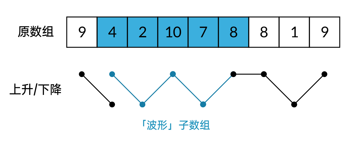
First, let’s understand what a “turbulent subarray” means. What we care about is the relative ordering between adjacent elements in the array. If the next element is greater than the previous one, it’s a “rising” segment of the array; otherwise, it’s a “falling” segment. A “turbulent subarray” is a subarray where rising and falling segments alternate. For example, in the input [9, 4, 2, 10, 7, 8, 8, 1, 9], [4, 2, 10, 7, 8] is the longest turbulent subarray.

Solving with a Single Subproblem

Let’s first see how to solve this problem using the traditional single-subproblem approach.

First, upon seeing the word “subarray” in the problem, we should immediately think of subarray-related techniques: when defining the subproblem, add the constraint that it must be at the tail of the array.

If you’re not familiar with this technique, you can review my previous article:

LeetCode Worked Examples | 16 Maximum Subarray Sum: Dynamic Programming Techniques for Subarray Problems

Using this technique, we can define the subproblem as follows:

Subproblem $f(k)$ represents “the longest turbulent subarray at the tail of array A[0..k).”

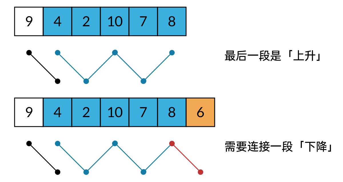
The reason we require the longest turbulent subarray to be at the tail of the array is that only a turbulent subarray at the tail can be extended by connecting a new rising/falling segment.

Note that connecting to a turbulent array is conditional — “rising” and “falling” segments must alternate. If the last segment of the turbulent array is “rising,” a “falling” segment must follow for it to remain a valid turbulent array; if the last segment is “falling,” a “rising” segment must follow.

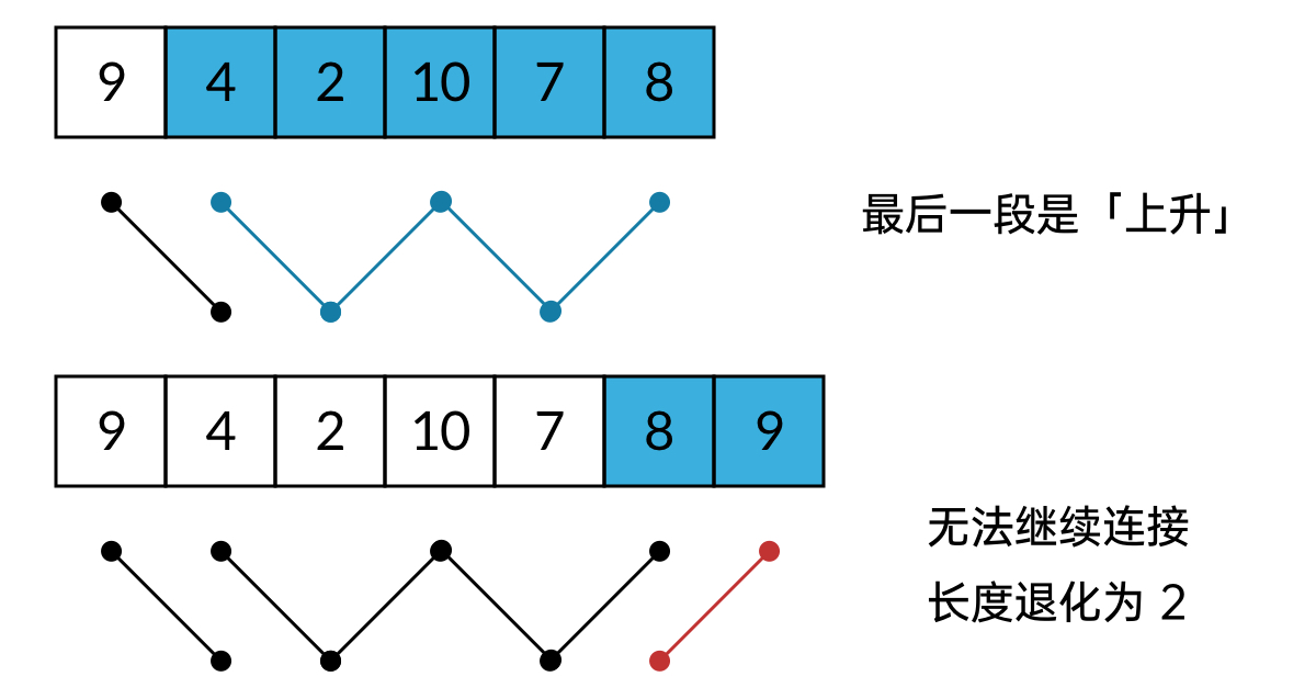
If “rising” is followed by another “rising,” the entire turbulent array becomes invalid. The turbulent subarray length shrinks to 2 (containing only the two elements of the last rising segment).

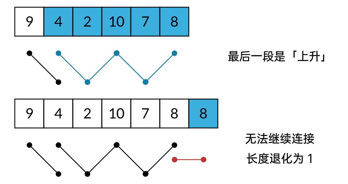
Of course, if the last segment is neither rising nor falling but “flat,” that last segment is also invalid. The turbulent subarray length shrinks to 1.

So when writing the recurrence relation, we need case analysis. For subproblem $f(k)$:

• If the last segment of $f(k-1)$‘s turbulent array is “rising” and the relationship between A[k-1] and A[k-2] is “rising,” then $f(k) = 2$;
• If the last segment of $f(k-1)$‘s turbulent array is “rising” and the relationship between A[k-1] and A[k-2] is “falling,” then $f(k) = f(k-1) + 1$;
• If the last segment of $f(k-1)$‘s turbulent array is “falling” and the relationship between A[k-1] and A[k-2] is “rising,” then $f(k) = f(k-1) + 1$;
• If the last segment of $f(k-1)$‘s turbulent array is “falling” and the relationship between A[k-1] and A[k-2] is “falling,” then $f(k) = 2$;
• If the relationship between A[k-1] and A[k-2] is “flat,” then $f(k) = 1$.

What? A seemingly simple problem requires this many cases? Getting dizzy yet?

Generally speaking, if you find the recurrence relation for a subproblem overly complex, it’s likely that the subproblem isn’t well-defined. Here’s the key insight: splitting the subproblem can eliminate a lot of unnecessary case analysis.

Below, we’ll try splitting the subproblem and solving with multiple subproblems.

Solving with Multiple Subproblems

Since we always need to check whether the last segment of the turbulent array is rising or falling, why not distinguish them right in the subproblem definition?

We can define two subproblems, corresponding to turbulent subarrays whose last segment is rising and falling, respectively:

• Subproblem $f(k)$ represents: the longest turbulent subarray at the tail of array A[0..k), with the last segment being “rising”;
• Subproblem $g(k)$ represents: the longest turbulent subarray at the tail of array A[0..k), with the last segment being “falling”.

With this, our recurrence relations become much clearer:

• If the relationship between A[k-1] and A[k-2] is “rising,” then $f(k) = g(k-1) + 1$, $g(k) = 1$;
• If the relationship between A[k-1] and A[k-2] is “falling,” then $f(k) = 1$, $g(k) = f(k-1) + 1$;
• If the relationship between A[k-1] and A[k-2] is “flat,” then $f(k) = 1$, $g(k) = 1$.

Now we can write the solution code. Note that since we defined multiple subproblems, we need to define multiple DP arrays in the code. We name the DP arrays f and g to match the subproblems:

public int maxTurbulenceSize(int[] A) {
    if (A.length <= 1) {
        return A.length;
    }

    int N = A.length;
    // Define two DP arrays f, g
    int[] f = new int[N+1];
    int[] g = new int[N+1];
    f[0] = 0;
    g[0] = 0;
    f[1] = 1;
    g[1] = 1;

    int res = 1;
    for (int k = 2; k <= N; k++) {
        if (A[k-2] < A[k-1]) {
            f[k] = g[k-1] + 1;
            g[k] = 1;
        } else if (A[k-2] > A[k-1]) {
            f[k] = 1;
            g[k] = f[k-1] + 1;
        } else {
            f[k] = 1;
            g[k] = 1;
        }
        res = Math.max(res, f[k]);
        res = Math.max(res, g[k]);
    }
    return res;
}

The Essence of Multiple Subproblems

Let’s understand what “defining multiple subproblems” really means in dynamic programming from the perspective of the DP array.

Consider this question: in the “Longest Turbulent Subarray” problem, is the DP array one-dimensional or two-dimensional?

From the subproblem definition, each subproblem has only one parameter $k$, so it appears to be one-dimensional. However, unlike typical one-dimensional DP problems, we have two subproblems $f(k)$ and $g(k)$, so there are two DP arrays, each of which is one-dimensional.

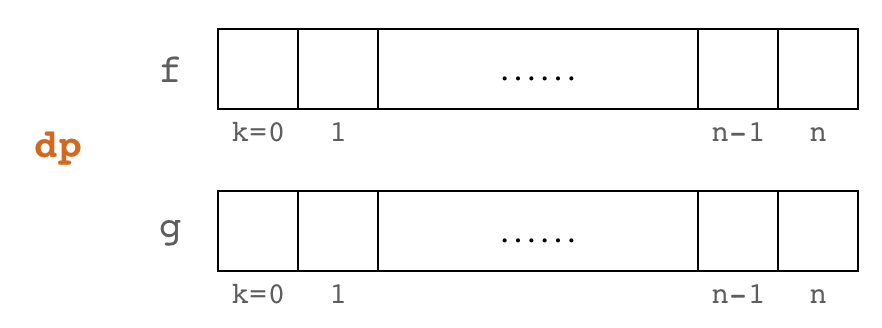
We can visualize the shape of the DP arrays to understand this intuitively. Let the array length be $n$. Then $k$ ranges over $[0, n]$. The DP arrays are two arrays of length $n+1$, as shown below.

Next, let’s draw the dependency relationships between subproblems in the DP arrays. $f(k)$ depends only on $g(k-1)$, and $g(k)$ depends only on $f(k-1)$, so the dependency relationships look like this:

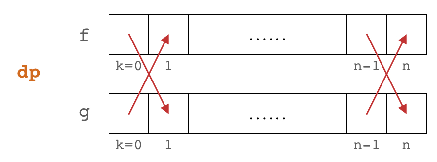
As we can see, the two subproblems depend on each other, and the overall dependency order goes from left to right.

On the other hand, we can also view the DP arrays as a two-dimensional array. Stacking the two arrays of length $n+1$ together gives a $2 \times (n+1)$ two-dimensional array.

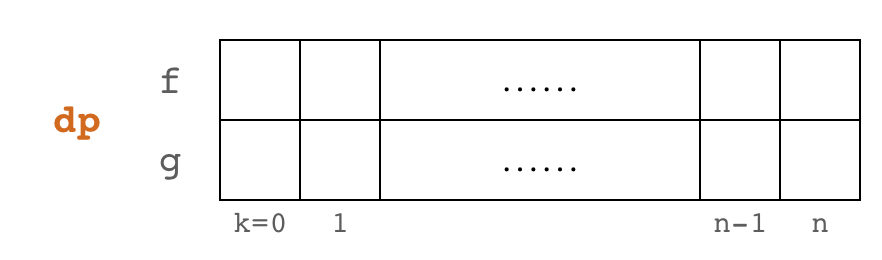
However, this DP array differs from the typical two-dimensional DP array in a few ways:

First, one dimension of the DP array has length 2, which is a constant. In terms of space complexity, this two-dimensional DP array has complexity $O(2n) = O(n)$, still at the one-dimensional level.

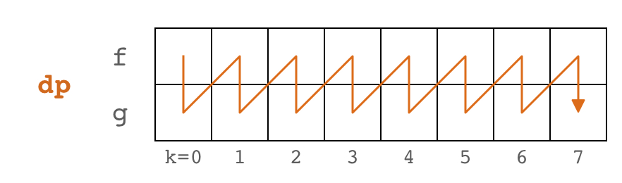
Second, in typical two-dimensional DP problems (like classic problems such as Longest Common Subsequence or Edit Distance), the DP array can be computed either top-to-bottom or left-to-right. But this DP array, based on its dependency order, can only be computed left-to-right — you cannot compute the first row ($f$) first and then the second row ($g$).

In summary, dynamic programming with multiple subproblems has a dimensionality that effectively lies between one-dimensional and two-dimensional. In this problem, we defined only two (a constant number of) subproblems, but if the number of subproblems scales up to $m$, the DP array’s space complexity reaches $O(mn)$, becoming a true two-dimensional DP problem.

Another Example: The Vacation Problem

Let’s look at another classic problem that involves splitting subproblems to understand the technique of defining multiple subproblems. This problem comes not from LeetCode, but from another algorithm site, AtCoder: AtCoder DP-C. Vacation

Problem link: https://atcoder.jp/contests/dp/tasks/dp_c

Taro’s summer vacation starts tomorrow, and he has decided to plan it out now.

The vacation lasts $N$ days. On day $i$ ($1 \le i \le N$), Taro can choose to do one of the following three activities:

• A: Swimming. Gain $a_i$ happiness points.
• B: Bug catching. Gain $b_i$ happiness points.
• C: Doing homework. Gain $c_i$ happiness points.

Since Taro gets bored easily, he cannot do the same activity on two consecutive days.

The input includes $N$ and the contents of arrays $a$, $b$, and $c$.

Calculate the maximum total happiness points Taro can earn.

How should we split the subproblems for this problem? We notice a key condition: Taro cannot do the same activity on two consecutive days. This means:

• If Taro does activity A today, he can do activities B and C tomorrow;
• If Taro does activity B today, he can do activities A and C tomorrow;
• If Taro does activity C today, he can do activities A and B tomorrow.

Based on which activity Taro does today, we can define three subproblems:

• Subproblem $f_1(k)$ represents the maximum happiness points Taro can earn in the first k days, given that he does activity A on day k;
• Subproblem $f_2(k)$ represents the maximum happiness points Taro can earn in the first k days, given that he does activity B on day k;
• Subproblem $f_3(k)$ represents the maximum happiness points Taro can earn in the first k days, given that he does activity C on day k.

Then we can write the recurrence relations between subproblems:

$$\begin{aligned} f_1(k) &= \max \{ f_2(k-1), f_3(k-1) \} + a_k \\ f_2(k) &= \max \{ f_1(k-1), f_3(k-1) \} + b_k \\ f_3(k) &= \max \{ f_1(k-1), f_2(k-1) \} + c_k \\ \end{aligned}$$

Why does the recurrence look like this? Let’s take the formula for $f_1(k)$ as an example:

$f_1(k)$ represents the maximum happiness points Taro can earn in the first k days, given that he does activity A on day k. Since Taro does activity A on day k, he cannot do activity A on day k-1 — he can only do activity B or C, corresponding to $f_2(k-1)$ and $f_3(k-1)$. In other words, $f_1(k)$ is derived from $f_2(k-1)$ and $f_3(k-1)$.

The formulas for $f_2(k)$ and $f_3(k)$ follow the same reasoning.

With this recurrence relation, we can write the solution code:

private static int vacation(int[] a, int[] b, int[] c) {
    int n = a.length;
    int[] f1 = new int[n+1];
    int[] f2 = new int[n+1];
    int[] f3 = new int[n+1];
    f1[0] = 0;
    f2[0] = 0;
    f3[0] = 0;
    for (int k = 1; k <= n; k++) {
        f1[k] = a[k-1] + Math.max(f2[k-1], f3[k-1]);
        f2[k] = b[k-1] + Math.max(f1[k-1], f3[k-1]);
        f3[k] = c[k-1] + Math.max(f1[k-1], f2[k-1]);
    }
    return Math.max(f1[n], Math.max(f2[n], f3[n]));
}

As you can see, the solution code is quite concise. In the code, f1, f2, and f3 exhibit a pattern of mutual dependency and alternating computation.

We can use the following diagram to describe the relationship among these three subproblems:

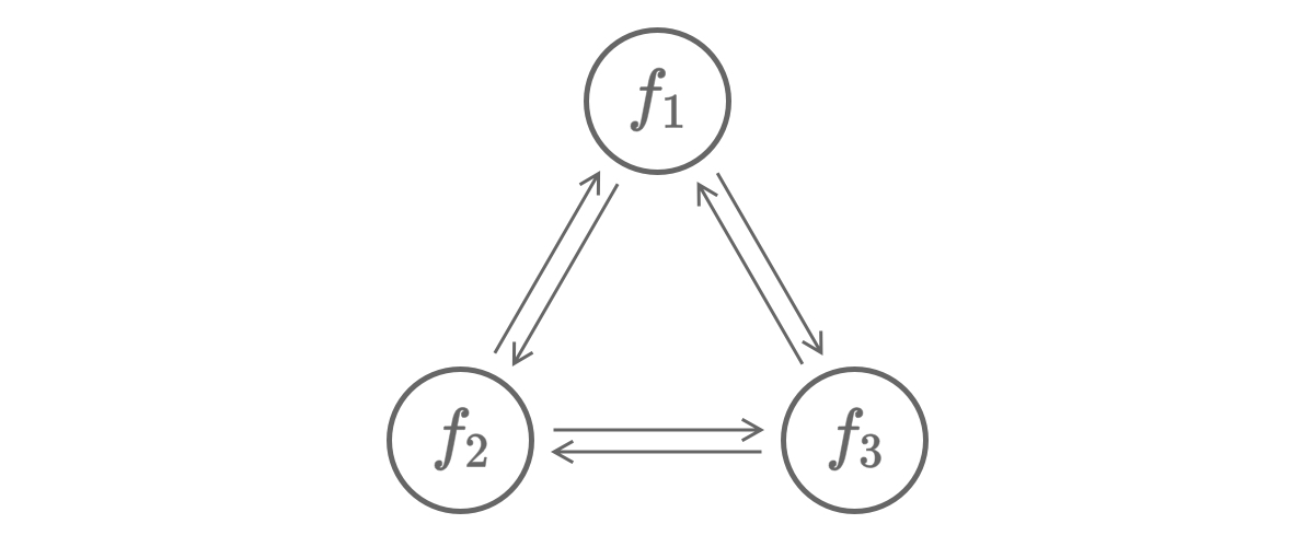
The arrows in the diagram represent dependency relationships between subproblems. For example, the edge from $f_1$ to $f_2$ means that $f_2(k)$ depends on $f_1(k-1)$. Since $f_1(k)$ does not depend on $f_1(k-1)$, there is no self-loop on $f_1$.

Sharp-eyed readers may have already noticed that this diagram actually depicts a state machine. The state machine has three states: $f_1$, $f_2$, and $f_3$. If the state machine is in state $f_1$ on day k-1, it cannot stay in $f_1$ on day k — it can only transition to $f_2$ or $f_3$. This corresponds to the problem’s condition that “Taro cannot do the same activity on two consecutive days.”

In fact, “state machine” is a technique in dynamic programming. The famous stock trading problem belongs to the “state machine DP” category. The next article will cover the stock trading problem and state machine DP in detail.

Summary

This article used two examples to demonstrate the technique of decomposing subproblems and defining multiple subproblems in dynamic programming. Although the two problems defined 2 and 3 subproblems respectively, the way subproblems are split and the computation order are very similar. Comparing these two problems side by side, you can quickly grasp the pattern of defining multiple subproblems in dynamic programming.

The famous stock trading problem is another common example of defining multiple subproblems. However, since the stock trading problem involves an important “state machine” definition step, it wasn’t the best fit as an example for this article.

In the next article, I’ll explain the approach to the stock trading problem in detail, focusing on how to add state machine reasoning on top of defining multiple subproblems. Stay tuned.