Longest Common Subsequence: Solving with Two-Dimensional Dynamic Programming - LeetCode by Example

Today’s problem: LeetCode 1143. Longest Common Subsequence (Medium)

Given two strings s and t, return the length of their longest common subsequence. If the two strings have no common subsequence, return 0.

A subsequence of a string is a new string generated from the original string with some characters (possibly none) deleted without changing the relative order of the remaining characters. For example, “ace” is a subsequence of “abcde”.

In the previous article, we used the House Robber problem as an example to explain the general steps for solving dynamic programming problems. However, the House Robber problem is a one-dimensional dynamic programming problem, and many other problems fall under two-dimensional dynamic programming. Today, we’ll use the classic “Longest Common Subsequence” problem to demonstrate how to solve two-dimensional DP problems.

How classic is the Longest Common Subsequence problem? Classic enough to have its own dedicated abbreviation — LCS (Longest Common Subsequence). If you see the abbreviation LCS elsewhere, you should know it refers to this problem.

If the House Robber problem is the best introductory problem for dynamic programming, then the LCS problem is the best introductory problem for two-dimensional dynamic programming — a classic problem with a quintessential approach. This article will walk through solving the LCS problem step by step, explaining the key techniques for two-dimensional DP problems along the way.

This article assumes you are already familiar with the House Robber solution and the basic steps for solving dynamic programming problems. If you need a refresher, check out the previous article:

LeetCode Problem Deep Dive | 14 House Robber: Four Steps to Solve Dynamic Programming Problems

One-Dimensional vs. Two-Dimensional Dynamic Programming

First, let’s clarify what one-dimensional and two-dimensional dynamic programming mean. For the House Robber problem, we defined $f(k)$ as the maximum amount from robbing the first $k$ houses. Here the subproblem has only one parameter $k$ , making it a one-dimensional DP problem where the parameter varies along a single dimension. If a subproblem has two parameters, it becomes a two-dimensional DP problem where parameters vary along two dimensions.

Why does the dimensionality of subproblems matter? Because the subproblem’s dimensionality directly affects the dimensionality of the DP array. A two-dimensional DP array not only increases space complexity, but also makes the computation order more complex.

Generally speaking, the vast majority of dynamic programming problems have dimensionality no greater than two. Problems that require three or more dimensions are considered hard problems and are not essential to master.

Solving with the Four-Step Approach

In the previous article, we introduced the four basic steps for solving dynamic programming problems:

Define the subproblem
Write the recurrence relation for the subproblem
Determine the computation order of the DP array
Space optimization (optional)

Two-dimensional DP problems follow the same four steps, though each step may be more complex. Let’s apply the four-step approach to solve the LCS problem step by step.

Step 1: Define the Subproblem

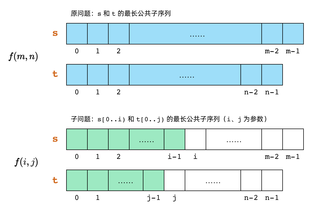
To define the subproblem, we rely on a fundamental property: a subproblem is similar to the original problem but smaller in scale. For the LCS problem, the original problem is “the longest common subsequence of s and t.” We can reduce the scale of either s or t, turning it into “the longest common subsequence of the first $i$ characters of s (s[0..i)) and the first $j$ characters of t (t[0..j))”, denoted as $f(i, j)$ . As you can see, the subproblem has two parameters $i$ and $j$ , making this a two-dimensional DP problem.

Subproblem definition for the LCS problem

Step 2: Write the Recurrence Relation

This is the most critical step in solving a dynamic programming problem. Two-dimensional subproblems can have many possible recurrence relations — some are immediately obvious, while others may require careful reasoning.

Generally, we first consider whether we can use the simplest type of recurrence: looking at the relationship between the current subproblem and the previous subproblem(s). For a one-dimensional subproblem, this means examining the relationship between $f(i)$ and $f(i-1)$ ; for a two-dimensional subproblem, it means examining the relationship between $f(i, j)$ and $f(i-1, j)$ , $f(i, j-1)$ , $f(i-1, j-1)$ . The LCS problem is a classic example of this simple recurrence pattern.

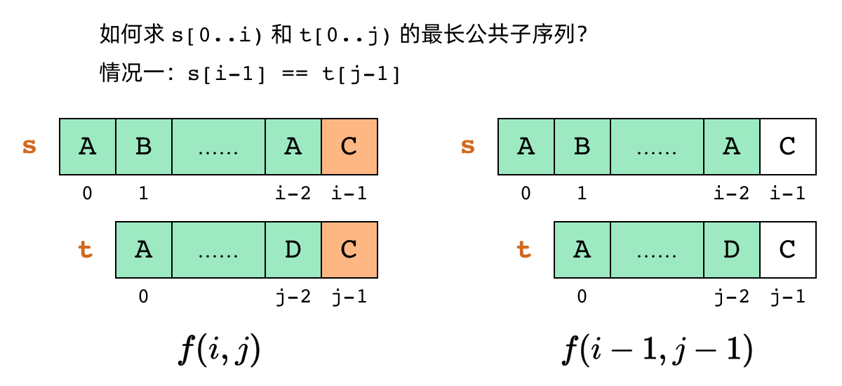
The subproblem $f(i, j)$ for the LCS problem represents “the longest common subsequence of s[0..i) and t[0..j).” We can compare the last characters of s and t, namely s[i-1] and t[j-1]. There are two possible cases:

Case 1: If s[i-1] == t[j-1], we can use this character as part of the longest common subsequence, then find the LCS of s[0..i-1) and t[0..j-1), as shown below.

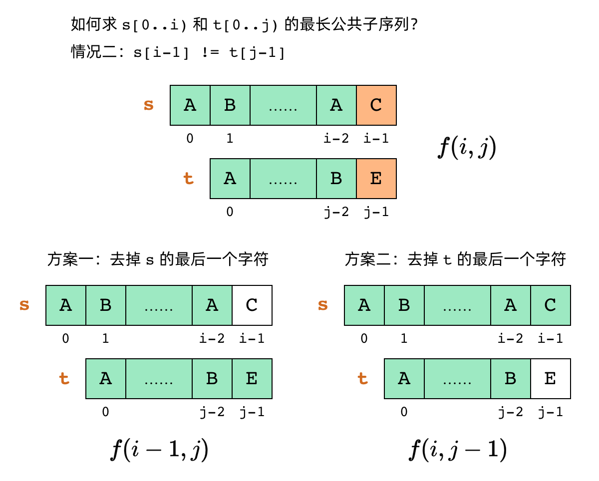
Case 2: If s[i-1] != t[j-1], we can try removing the last character from either s or t — that is, compare s[0..i-1) with t[0..j), or compare s[0..i) with t[0..j-1) — and choose whichever yields the longer common subsequence, as shown below.

This gives us the following recurrence relation:

f(i, j) = \begin{cases} f(i-1, j-1) + 1, & \text{if } s_{i-1} = t_{j-1} \\ \max \begin{cases} f(i-1, j) \\ f(i, j-1) \\ \end{cases}, & \text{if } s_{i-1} \ne t_{j-1} \\ \end{cases}

We also need to specify the base cases. When $i = 0$ , s[0..i) is empty, so the LCS length of s[0..i) and t[0..j) is $0$ . Therefore $f(0, j) = 0$ . Similarly, when $j=0$ , t[0..j) is empty, so $f(i, 0) = 0$ .

Step 3: Determine the Computation Order of the DP Array

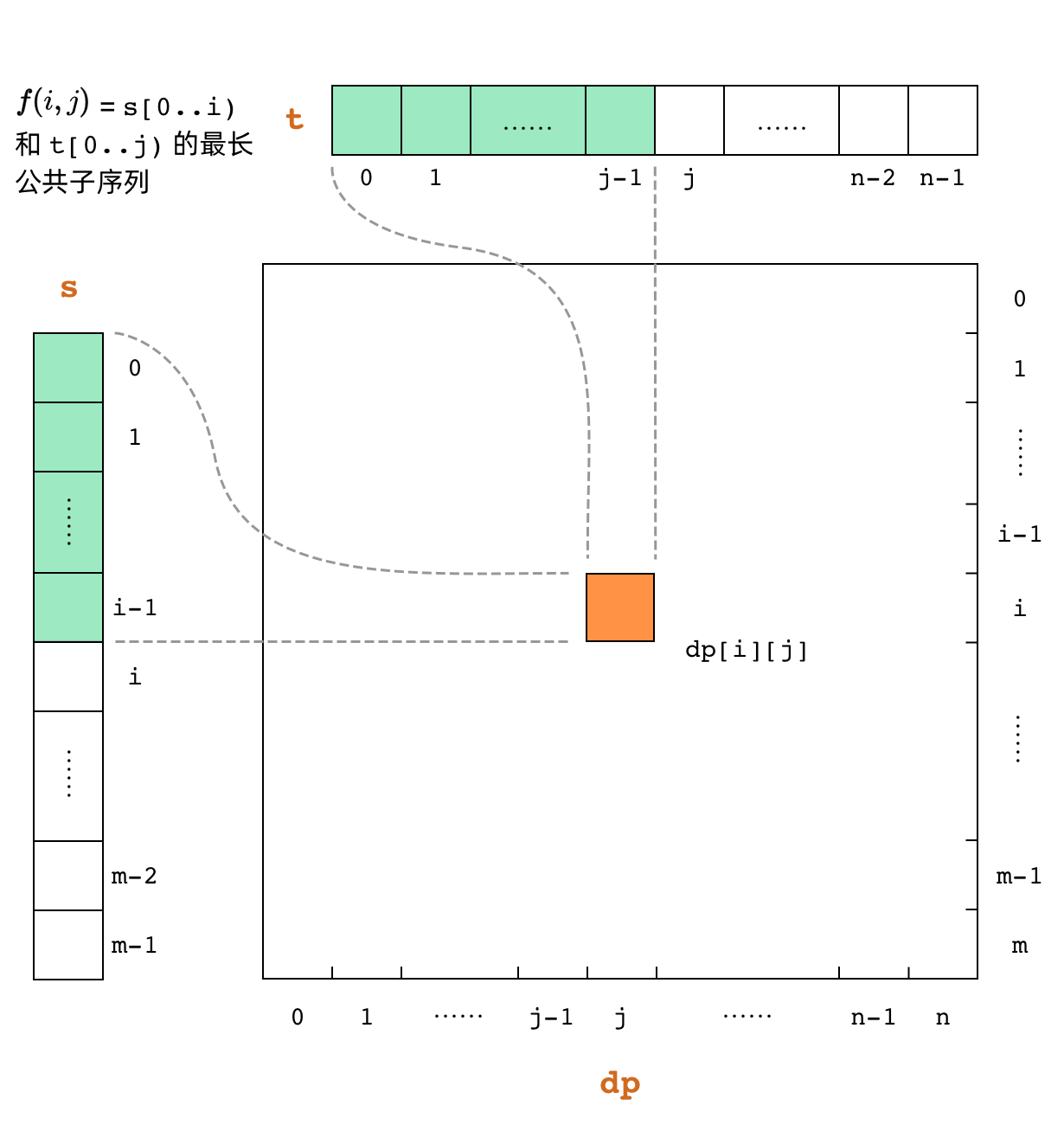
For two-dimensional DP problems, we still use a DP array and compute subproblems in a bottom-up fashion. Since each element in the DP array corresponds to a subproblem, when the subproblems become two-dimensional, the DP array also needs to be a two-dimensional array. In the DP array, dp[i][j] corresponds to subproblem $f(i, j)$ , which is the LCS of s[0..i) and t[0..j), as shown below.

Correspondence between the DP array and subproblems

In the previous article on the House Robber problem, we directly stated that the DP array should be computed from left to right. For one-dimensional DP problems, we can determine the computation order intuitively. However, for two-dimensional DP problems, we need a more systematic way to figure out the computation order.

The fundamental principle for the DP array computation order is: when we compute a subproblem, all subproblems it depends on should already be computed. Based on this principle, let’s consider three things.

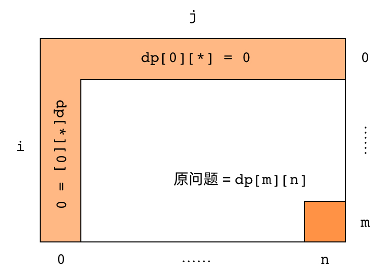
First: What is the valid range of the DP array? Let the length of s be $m$ and the length of t be $n$ . Then the ranges for $i$ and $j$ are: $0 \le i \le m, \; 0 \le j \le n$ . So when declaring the DP array, we should write:

int[][] dp = new int[m+1][n+1];

The entire rectangular region of the two-dimensional DP array is valid.

Second: Where are the base cases and the original problem in the DP array? As shown below, the base cases are located in the leftmost column and topmost row of the DP array, while the original problem is in the bottom-right corner.

Positions of base cases and original problem in the DP array

Third: What is the dependency direction of subproblems in the DP array? Looking at the recurrence relation, $f(i, j)$ depends on $f(i-1, j)$ , $f(i, j-1)$ , and $f(i-1, j-1)$ . Let’s draw the relationship between dp[i][j] and dp[i-1][j], dp[i][j-1], dp[i-1][j-1], with arrows showing the dependency direction:

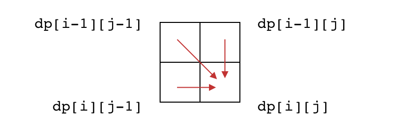
We can see that the dependency direction goes rightward and downward, so the computation order should also be left to right, top to bottom. In other words, we should iterate through the DP array like this:

for (int i = 0; i <= m; i++) {
    for (int j = 0; j <= n; j++) {
        // compute dp[i][j] ...
    }
}

Inside the loop, we simply fill in the recurrence relation. With this, we can easily write the solution:

public int longestCommonSubsequence(String s, String t) {
    if (s.isEmpty() || t.isEmpty()) {
        return 0;
    }
    // Subproblem:
    // f(i, j) = LCS of s[0..i) and t[0..j)

    // f(0, *) = 0
    // f(*, 0) = 0
    // f(i, j) = f(i-1, j-1) + 1, if s[i-1] == t[j-1]
    //           max{ f(i-1, j), f(i, j-1) }, otherwise

    int m = s.length();
    int n = t.length();
    int[][] dp = new int[m+1][n+1];
    for (int i = 0; i <= m; i++) {
        for (int j = 0; j <= n; j++) {
            if (i == 0 || j == 0) {
                dp[i][j] = 0;
            } else {
                if (s.charAt(i-1) == t.charAt(j-1)) {
                    dp[i][j] = dp[i-1][j-1] + 1;
                } else {
                    dp[i][j] = Math.max(dp[i-1][j], dp[i][j-1]);
                }
            }
        }
    }
    return dp[m][n];
}

Note that the code above includes a large block of comments about the subproblem definition and recurrence relation. During interviews, it’s best to write these out — it gives you a reference while coding and helps the interviewer follow your thought process.

Step 4: Space Optimization (Optional)

For two-dimensional DP problems, the DP array becomes a two-dimensional array with higher space complexity. Therefore, space optimization is even more worthwhile for two-dimensional DP problems to reduce space complexity.

However, there are many different space optimization techniques for two-dimensional DP problems, and you need to apply them flexibly depending on the situation. The space optimization step is optional — you can skip it. I’ll write a dedicated article later covering various space optimization techniques.

For this LCS problem, here is the space-optimized code using a one-dimensional array plus a temporary variable. If you’re curious, try to figure out why this optimization works.

public int longestCommonSubsequence(String s, String t) {
    if (s.isEmpty() || t.isEmpty()) {
        return 0;
    }

    int m = s.length();
    int n = t.length();
    int[] dp = new int[n+1]; // newly allocated array is initialized to 0 by default
    for (int i = 1; i <= m; i++) {
        int temp = 0;
        for (int j = 1; j <= n; j++) {
            int dp_j;
            if (s.charAt(i-1) == t.charAt(j-1)) {
                dp_j = temp + 1;
            } else {
                dp_j = Math.max(dp[j], dp[j-1]);
            }
            temp = dp[j];
            dp[j] = dp_j;
        }
    }
    return dp[n];
}

Note that space optimization can only reduce space complexity, not time complexity. For example, the complexity of the LCS problem before and after optimization is:

Before optimization: time complexity $O(n^2)$ , space complexity $O(n^2)$ .
After optimization: time complexity $O(n^2)$ , space complexity $O(n)$ .

Summary

This article used the Longest Common Subsequence (LCS) problem to demonstrate the basic approach to two-dimensional dynamic programming. Regardless of whether a DP problem is one-dimensional or two-dimensional, the four basic steps always apply, and we should keep them in mind when solving problems.

Compared to one-dimensional DP, the most complex aspects of two-dimensional DP lie in the recurrence relation and the computation order. As an introductory problem, the LCS problem has a fairly standard computation order. Later topics on “Interval DP” and “Knapsack DP” will really open your mind to new possibilities.

Many two-dimensional DP problems share similarities with the LCS problem. For example, the “Edit Distance” problem has a somewhat different derivation, but its overall approach and subproblem dependency pattern are very similar to LCS. Another example is the “Longest Palindromic Subsequence” problem, which looks like the LCS subproblem dependency direction rotated by some angle. We’ll cover all of these problem types in upcoming articles.