A Practical yet Elegant Approach to Stock Trading Problems

The “stock trading problem” is probably one of the biggest roadblocks every LeetCode enthusiast runs into, especially the third problem in the series. Have you ever been stumped by it too?

There are six stock trading problems on LeetCode, forming an impressive series. The first two problems are not that hard — you can arrive at solutions through some clever thinking. However, just when you think the whole series can be tackled incrementally, the third problem ramps up the difficulty dramatically, catching you completely off guard.

What’s even more frustrating is that when you open the discussion section for this tough problem, you see an impossibly slick solution like this:

public int maxProfit(int[] prices) {
    if (prices.length == 0) return 0;
    int s1 = Integer.MIN_VALUE, s2 = 0,
        s3 = Integer.MIN_VALUE, s4 = 0;
    for (int p : prices) {
        s1 = Math.max(s1, -p);
        s2 = Math.max(s2, s1 + p);
        s3 = Math.max(s3, s2 - p);
        s4 = Math.max(s4, s3 + p);
    }
    return Math.max(0, s4);
}

WTF?? What’s the deal with these cryptic four variables s1/s2/s3/s4? How does this computation even capture the “at most two transactions” constraint?

Don’t panic. There’s actually a pattern to these problems, and once you master it, you’ll be able to write equally elegant solutions yourself. This pattern is also highly practical — it can be used to solve all the stock trading problems in the series.

Today, let me walk you through this practical yet elegant approach step by step. This article will cover the key techniques involved in the stock trading solution:

• State decomposition and state machine definition for DP subproblems
• Special value definitions for the DP array
• Space optimization techniques for dynamic programming

Solution

Let’s solve the most representative stock problem (III), which serves as the foundation for the other problems in the series:

LeetCode 123. Best Time to Buy and Sell Stock III (Hard)

Given an array where the $i$-th element is the price of a given stock on day $i$, design an algorithm to find the maximum profit. You may complete at most two transactions.

Note: You may not engage in multiple transactions simultaneously (you must sell the stock before you buy again).

Example:

text

Input: [3,3,5,0,0,3,1,4]
Output: 6
Explanation: Buy on day 4 (price = 0) and sell on day 6 (price = 3), profit = 3-0 = 3.
     Then buy on day 7 (price = 1) and sell on day 8 (price = 4), profit = 4-1 = 3.

Many of you may have a vague sense that this problem calls for dynamic programming, but can’t quite figure out a concrete approach.

The biggest challenge of this problem lies in its constraint: “at most two transactions.” How do we express this constraint in dynamic programming? How do we track the “different states” throughout the stock trading process? The answer lies entirely in the technique we discussed in the previous article: decomposing DP subproblems.

If you need a refresher on the previous article, click here:

LeetCode Problem Analysis | 17: How to Decompose Subproblems in Dynamic Programming to Simplify Your Approach

Of course, if you just want to know the solution to the stock trading problem, feel free to read on.

State Machine Definition

For the constraint “at most two transactions,” we can think of it as: the stock trading process goes through different phases.

• At the beginning, the constraint is “at most two transactions”;
• After completing one transaction, the constraint becomes “only one transaction left”;
• After completing two transactions, the constraint becomes “no more transactions allowed.”

Some solutions define a parameter $k$ to represent the number of remaining transactions. But since $k$ only takes values 2, 1, and 0, adding an extra dimension to the DP just for that isn’t worthwhile. Instead, we can directly define multiple subproblems to describe these different phases.

Additionally, the problem states “you must sell the stock before buying again,” which further divides the trading process into phases. We have two states: “holding stock” and “not holding stock.” When holding stock, we can only sell, not buy. When not holding stock, it’s the opposite.

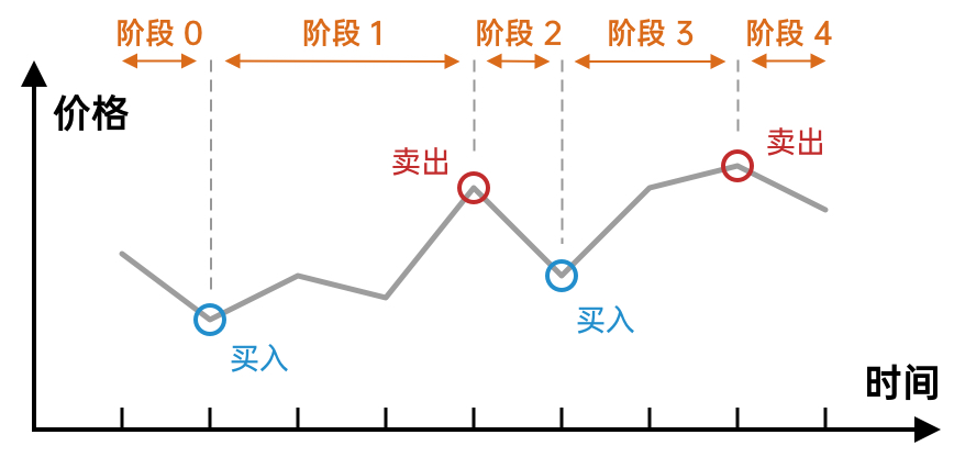
Overall, with two transactions, the stock trading process can be divided into five phases:

Corresponding to these five phases, we define five subproblems represented by $s_0$, $s_1$, $s_2$, $s_3$, $s_4$. The letter s stands for state — the transitions between stock trading phases are essentially state transitions.

For example, in phase 1, we are holding stock. If we sell the stock at this point, we transition to a state where we no longer hold stock, entering phase 2.

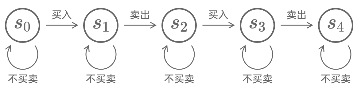
The state transitions among $s_0$ through $s_4$ can be illustrated with the following diagram:

On each day, we can either choose to buy/sell or choose to do nothing. If we buy or sell, we advance to the next phase, corresponding to the rightward edges in the state transition diagram; if we do nothing, we stay in the current phase, corresponding to the self-loops in the diagram.

This is what’s known as “State Machine DP.” Defining multiple subproblems, from another perspective, means the subproblems jump between different “states.”

Now that we understand the relationships between subproblems, let’s formally define them and their recurrence relations: subproblems $s_{0/1/2/3/4}(k)$ represent “the maximum profit at the end of the first $k$ days when in phase 0/1/2/3/4.” Then we have:

• $s_0(k) = 0$. Because in phase 0, no buying or selling has occurred.
• $s_1(k) = \max \{ s_1(k-1), s_0(k-1) - p_k \}$. Being in phase 1 on day k means either we were in phase 1 the day before, or we were in phase 0 and bought the stock on day k (profit decreases by $p_k$).
• $s_2(k) = \max \{ s_2(k-1), s_1(k-1) + p_k \}$. Being in phase 2 on day k means either we were in phase 2 the day before, or we were in phase 1 and sold the stock on day k (profit increases by $p_k$).
• $s_3(k) = \max \{ s_3(k-1), s_2(k-1) - p_k \}$. The analysis is the same as $s_1(k)$.
• $s_4(k) = \max \{ s_4(k-1), s_3(k-1) + p_k \}$. The analysis is the same as $s_2(k)$.

Understanding the DP Array

After defining the subproblems and their recurrence relations, we still need to figure out the computation order of the DP array.

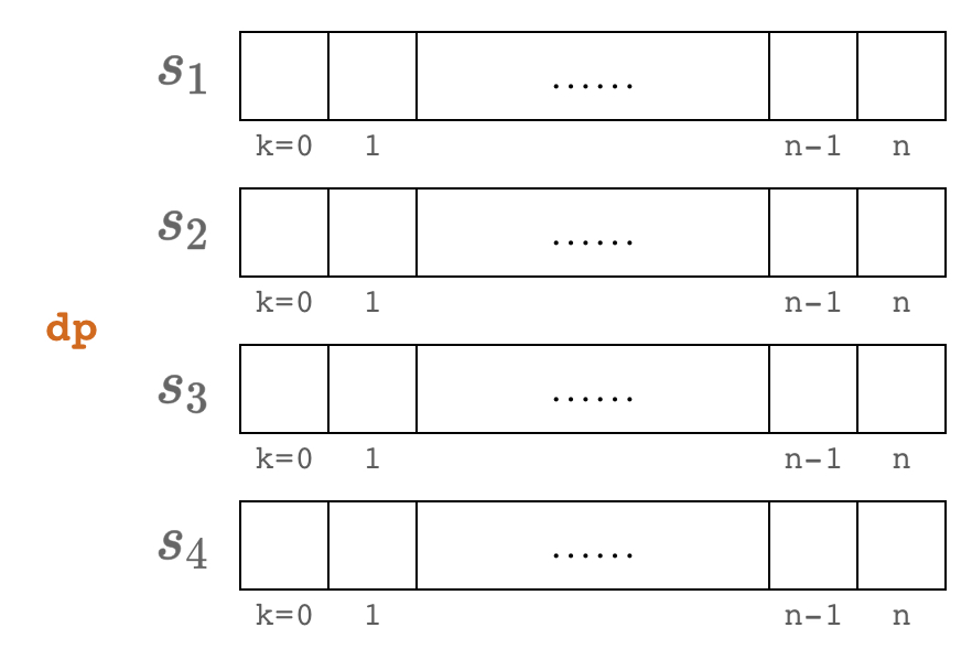
First, since $s_0$ is always 0, we don’t actually need to compute it — we can just substitute it as the constant 0. This leaves us with only the four subproblems $s_1$/$s_2$/$s_3$/$s_4$.

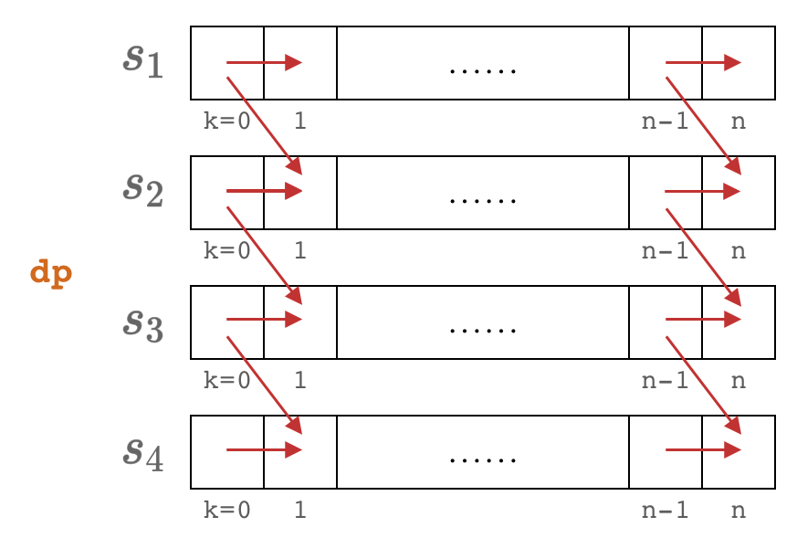
For all four subproblems, $k$ ranges from $0 \le k \le n$. So our DP array consists of four one-dimensional arrays of length $n+1$, as shown below.

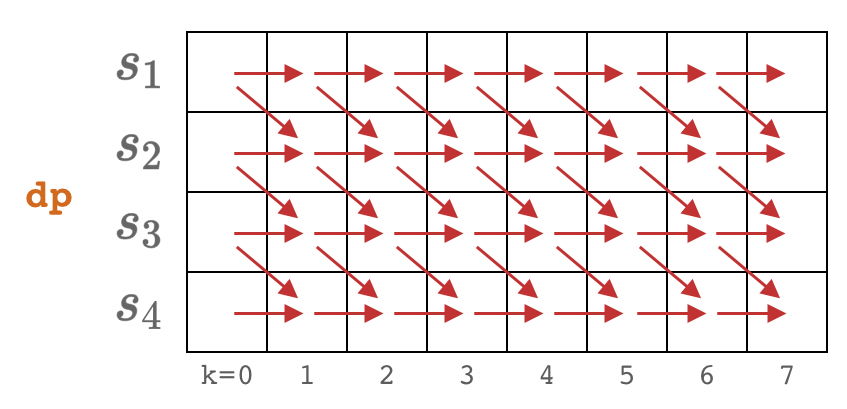
Next, let’s look at the dependencies in the DP array:

As we can see, the DP array is computed from left to right and top to bottom. Based on this, we can write the initial solution code:

// Note: this code is not yet complete
public int maxProfit(int[] prices) {
    if (prices.length == 0) {
        return 0;
    }

    int n = prices.length;
    int[] s1 = new int[n+1];
    int[] s2 = new int[n+1];
    int[] s3 = new int[n+1];
    int[] s4 = new int[n+1];
    // Note: base case assignments are still missing here
    for (int k = 1; k <= n; k++) {
        s1[k] = Math.max(s1[k-1], -p[k-1]);
        s2[k] = Math.max(s2[k-1], s1[k-1] + p[k-1]);
        s3[k] = Math.max(s3[k-1], s2[k-1] - p[k-1]);
        s4[k] = Math.max(s4[k-1], s3[k-1] + p[k-1]);
    }
    return Math.max(0, Math.max(s2[n], s4[n]));
}

Handling the Base Case

The code above isn’t quite complete yet — we still need to fill in the base case values for the subproblems.

For this problem, determining the base case values isn’t straightforward. The difficulty lies in the fact that some elements in the DP array are invalid.

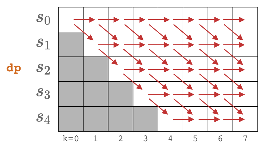
Take $s_2$ as an example. $s_2(0)$ should represent: the maximum profit after one buy and one sell at day 0 (i.e., the very beginning). But obviously we can’t perform any transactions on day 0, so $s_2(0)$ is an invalid element. We can deduce that $s_2$ is only valid for $k \ge 2$.

By the same reasoning, we can determine that the base cases for $s_1$, $s_2$, $s_3$, $s_4$ are $s_1(1)$, $s_2(2)$, $s_3(3)$, $s_4(4)$ respectively, as shown below (including $s_0$ here for clarity).

If we used conditional checks to handle these invalid elements, the code would become very complex. Is there a better way?

The answer is to assign special values to $s_1(0)$, $s_2(0)$, $s_3(0)$, $s_4(0)$. While these values have no practical meaning, they won’t affect the computation of valid values later, nor will they affect the final result.

Since the final result asks for the maximum profit (max), we can assign these invalid elements a value smaller than any possible result:

• For $s_2$ and $s_4$, this value is $0$. Because these two states don’t hold stock, and valid values obviously won’t be less than 0 (you can simply not trade, and the profit is 0).
• For $s_1$ and $s_3$, this value is $-\infty$. Because these two states require holding stock, and buying results in a temporary negative profit.

After adding these base cases, we get the complete code:

public int maxProfit(int[] prices) {
    if (prices.length == 0) {
        return 0;
    }

    int n = prices.length;
    int[] s1 = new int[n+1];
    int[] s2 = new int[n+1];
    int[] s3 = new int[n+1];
    int[] s4 = new int[n+1];
    s1[0] = Integer.MIN_VALUE;
    s2[0] = 0;
    s3[0] = Integer.MIN_VALUE;
    s4[0] = 0;
    for (int k = 1; k <= n; k++) {
        s1[k] = Math.max(s1[k-1], -prices[k-1]);
        s2[k] = Math.max(s2[k-1], s1[k-1] + prices[k-1]);
        s3[k] = Math.max(s3[k-1], s2[k-1] - prices[k-1]);
        s4[k] = Math.max(s4[k-1], s3[k-1] + prices[k-1]);
    }
    return Math.max(0, Math.max(s2[n], s4[n]));
}

Space Optimization

The code above is already fairly clean, but it still differs slightly from the ultra-concise version we showed at the beginning. Next, let’s apply a space optimization technique to make it even more compact.

Let’s revisit the DP array dependency diagram:

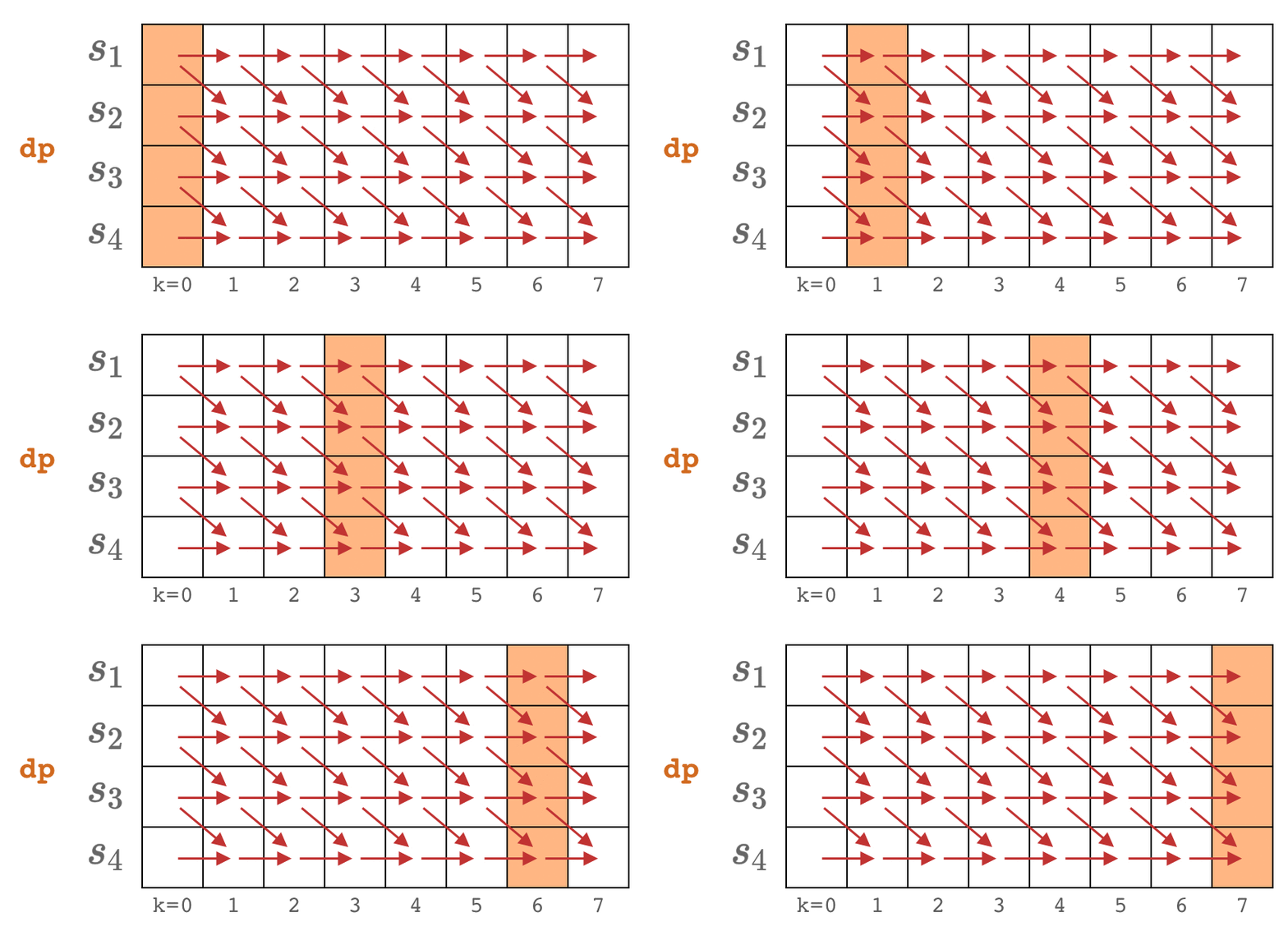
We notice that each column’s values depend only on the previous column’s values. This means we only need to keep the current column’s values and compute the next column in each iteration.

This way, s1, s2, s3, s4 go from one-dimensional arrays to single variables.

int s1 = Integer.MIN_VALUE;
int s2 = 0;
int s3 = Integer.MIN_VALUE;
int s4 = 0;
for (int k = 1; k <= n; k++) {
    s4 = Math.max(s4, s3 + prices[k-1]);
    s3 = Math.max(s3, s2 - prices[k-1]);
    s2 = Math.max(s2, s1 + prices[k-1]);
    s1 = Math.max(s1, -prices[k-1]);
}

The code above has prices[k-1] appearing everywhere. Let’s replace k-1 with k:

int s1 = Integer.MIN_VALUE;
int s2 = 0;
int s3 = Integer.MIN_VALUE;
int s4 = 0;
for (int k = 0; k < n; k++) {
    s4 = Math.max(s4, s3 + prices[k]);
    s3 = Math.max(s3, s2 - prices[k]);
    s2 = Math.max(s2, s1 + prices[k]);
    s1 = Math.max(s1, -prices[k]);
}

Then convert the for loop to a for-each loop:

int s1 = Integer.MIN_VALUE;
int s2 = 0;
int s3 = Integer.MIN_VALUE;
int s4 = 0;
for (int p : prices) {
    s4 = Math.max(s4, s3 + p);
    s3 = Math.max(s3, s2 - p);
    s2 = Math.max(s2, s1 + p);
    s1 = Math.max(s1, -p);
}

And there we have the final simplified code:

public int maxProfit(int[] prices) {
    if (prices.length == 0) {
        return 0;
    }

    int s1 = Integer.MIN_VALUE;
    int s2 = 0;
    int s3 = Integer.MIN_VALUE;
    int s4 = 0;
    for (int p : prices) {
        s4 = Math.max(s4, s3 + p);
        s3 = Math.max(s3, s2 - p);
        s2 = Math.max(s2, s1 + p);
        s1 = Math.max(s1, -p);
    }
    return Math.max(0, Math.max(s2, s4));
}

Following along step by step, doesn’t that intimidating code from the beginning seem much more approachable now?

Summary

This article dissected the stock trading problem’s solution technique step by step. If you look at the final code directly, you might feel it’s too clever and give up on the problem. But following the thought process in this article, you’ll find that the code actually evolved into this form through a series of simplifications.

Many answers in LeetCode’s discussion section love to show off code brevity and compete on line count. But pursuing minimal code isn’t helpful for truly understanding the problem. For this problem, what’s most worth mastering is actually the version without space optimization — the one that defines four one-dimensional arrays. Especially in interviews, if you write the space-optimized ultra-concise code right away, the interviewer might think you just “memorized the solution,” which could actually leave a bad impression.

The approach described in this article is sometimes called “State Machine DP.” The key to this approach is defining multiple subproblems and then describing the state transition relationships between them. After reading this article, I strongly recommend connecting the stock trading problem with the examples from the previous article — it will give you a much deeper understanding of this class of problems.

The other problems in the stock trading series can also be solved using the same technique. In upcoming articles, I’ll show you how to extend “at most two transactions” to the general case of “at most k transactions,” as well as how to handle variants with transaction fees and cooldown periods. Stay tuned.